はじめに
今回も前回に引き続き自作プログラムでベーシックな画像処理まがいのことをしていきます.
今回のお品書きはこちらです.
- カラーヒストグラム表示
- RGB→HSV変換とHSV→RGBのマッピング
- トーンカーブ機能の作成
その1. カラーヒストグラムの表示
RGB 3チャンネルではなく1チャンネルのみのヒストグラムは既にできていたので,ちょちょっと改造です.カラー画像と認識したデータに対する出力の右側にヒストグラムを表示するようにしました.
pub(crate) fn show_hist_color(&self, ui: &Ui, pos: [f32; 2], size: [f32; 2]) {
  let vmin = 0.0;
  let vmax = 65535.0;

  const FILL_COLOR_R: u32 = 0x5500_00FF;
  const FILL_COLOR_G: u32 = 0x5500_FF00;
  const FILL_COLOR_B: u32 = 0x55FF_0000;
  const BORDER_COLOR: u32 = 0xFF00_0000;
  let hist = self.image.hist_color();
  if let Some((max_count_r, max_count_g, max_count_b)) = hist
      .iter()
      .map(|bin| (bin[0].count, bin[1].count, bin[2].count))
      .max()
  {
    let draw_list = ui.get_window_draw_list();
    let max_count = max_count_r.max(max_count_g).max(max_count_b);
    let x_pos = pos[0];
    for i in 0..3 {
      for bin in hist {
        let y_pos = pos[1] + size[1] / (vmax - vmin) * (vmax - bin[i].start);
        let y_pos_end = pos[1] + size[1] / (vmax - vmin) * (vmax - bin[i].end);
        let length = size[0]
          * if self.hist_logscale {
            (bin[i].count as f32).log10() / (max_count as f32).log10()
          } else {
            (bin[i].count as f32) / (max_count as f32)
          };
          draw_list
            .add_rect(
              [x_pos + size[0] - length, y_pos],
              [x_pos + size[0], y_pos_end],
              if i == 0 {
                FILL_COLOR_R
              } else if i == 1 {
                FILL_COLOR_G
              } else {
                FILL_COLOR_B
              },
            )
            .filled(true)
            .build();
      }
    }
    draw_list
      .add_rect(pos, [pos[0] + size[0], pos[1] + size[1]], BORDER_COLOR)
      .build();
  }
}
するとこんな感じにカラー画像の横に出てきます.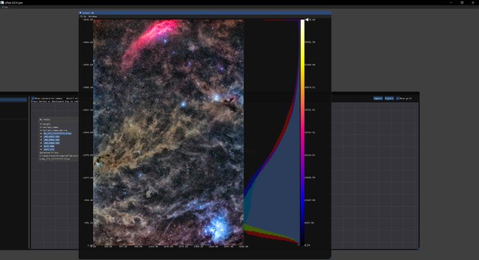
その2. RGB→HSV変換
このサイトによると,画素の RGB それぞれの輝度値$$R, G, B$$として,
$$Max = \max(R, G, B), Min = \min(R, G, B)$$
$$H = 60 * ((G - B) / (Max - Min)) ,; \max(R, G, B) = R$$
$$H = 60 * ((B - R) / (Max - Min)) + 120 ,; \max(R, G, B) = G$$
$$H = 60 * ((R - G) / (Max - Min)) + 240 ,; \max(R, G, B) = B$$
$$S = (Max - Min) / Max$$
$$V = Max$$
と計算できるっぽいのでこれに習っていきます.上の例だと色相は360度で表現してますが,後々 RGB に再マッピングすることを考えて 16bit の範囲に再スケールしておきます.
fn run_color_image_to_hsv(image: &WcsArray) -> Result<IOValue, IOErr> {
  dim_is!(image, 3)?;
  let image = image.scalar();
  let mut out = image.clone();
  for (j, slice) in image.axis_iter(Axis(1)).enumerate() {
    for (i, data) in slice.axis_iter(Axis(1)).enumerate() {
      let mut hue = 0.0;
      let max = data[0].max(data[1]).max(data[2]);
      let min = data[0].min(data[1]).min(data[2]);
      if data[0] >= data[1] && data[0] >= data[2] {
        hue = 60.0 * ((data[1] - data[2]) / (max - min));
      } else if data[1] >= data[0] && data[1] >= data[2] {
        hue = 60.0 * ((data[2] - data[0]) / (max - min)) + 120.0;
      } else if data[2] >= data[0] && data[2] >= data[1] {
        hue = 60.0 * ((data[0] - data[1]) / (max - min)) + 240.0;
      } else {
        println!("Unreachable");
      }
      if hue < 0.0 {
        hue += 360.0;
      }
      hue = hue / 360.0 * 65535.0;
      out[[0, j, i]] = hue;
      out[[1, j, i]] = (max - min) / max * 65535.0;
      out[[2, j, i]] = max;
    }
  }
  Ok(IOValue::Image(WcsArray::from_array(Dimensioned::new(
    out,
    Unit::None,
  ))))
}
まずは HSV の値が入っている三次元データをスライスして見てみるとこんな感じの強度分布図になります.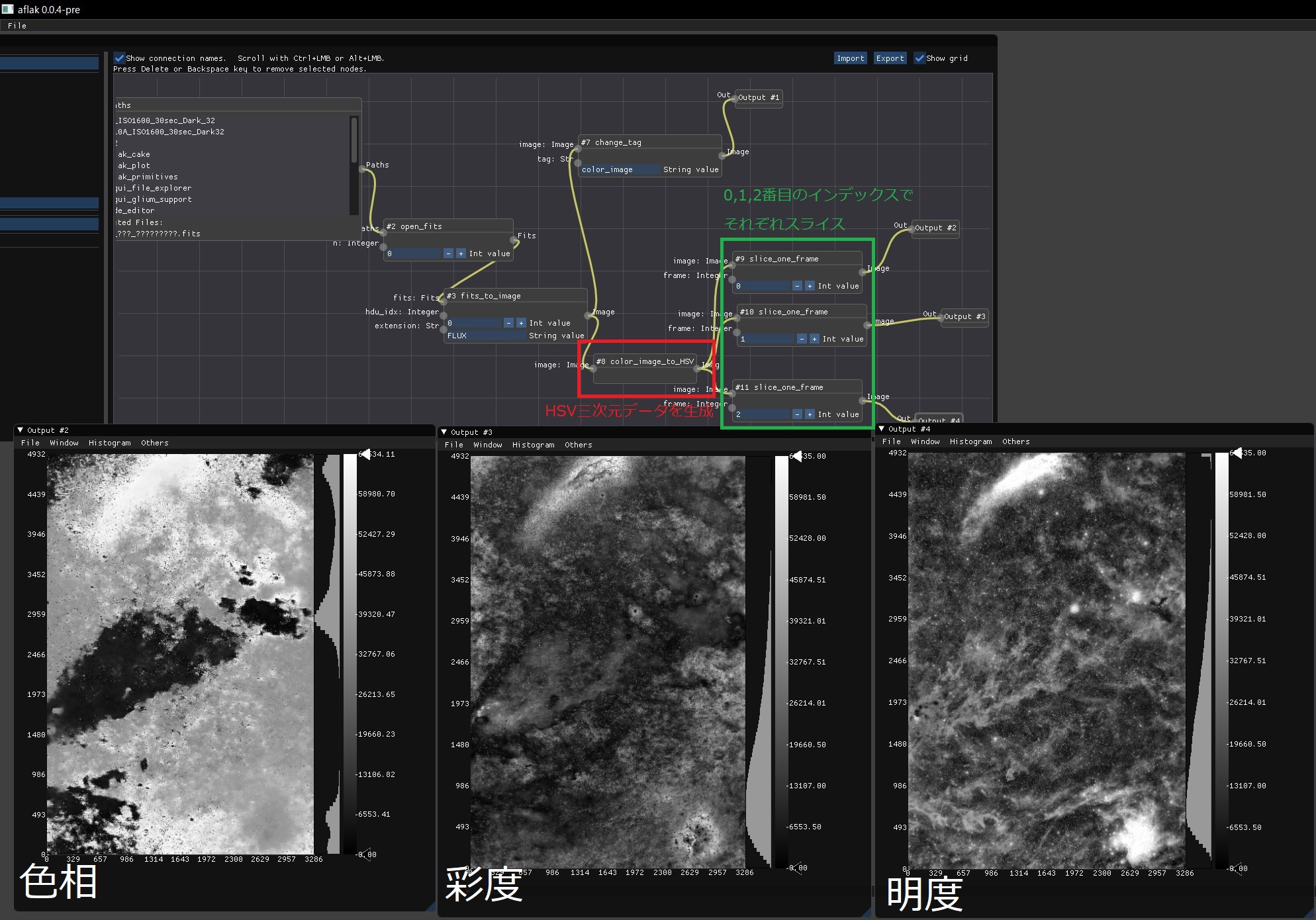
上のビジュアルプログラムについて少し説明を書いておくと,まず上記の計算式から 0番目に色相のマップ,1番目に彩度のマップ,2番目に明度のマップが入っているような三次元データを作ります(図の赤枠).この三次元データは右側に流れていき,スライスすることでそれぞれのマップデータ(二次元)を得ています.
次にこれらをRGBに再マッピングしてみます.次のような,三つの二次元のチャンネルデータを受け取ってカラー画像(三次元データ)を出力するようなノードを作ります.
fn run_generate_color_image_from_channel(
    image_r: &WcsArray,
    image_g: &WcsArray,
    image_b: &WcsArray,
) -> Result<IOValue, IOErr> {
  dim_is!(image_r, 2)?;
  dim_is!(image_g, 2)?;
  dim_is!(image_b, 2)?;
  are_same_dim!(image_r, image_b)?;
  are_same_dim!(image_b, image_g)?;
  let dim = image_r.scalar().dim();
  let dim = dim.as_array_view();
  let mut colorimage = Vec::with_capacity(3 * dim[0] * dim[1]);
  for &data in image_r.scalar().iter() {
    colorimage.push(data);
  }
  for &data in image_g.scalar().iter() {
    colorimage.push(data);
  }
  for &data in image_b.scalar().iter() {
    colorimage.push(data);
  }
  let img = Array::from_shape_vec((3, dim[0], dim[1]), colorimage).unwrap();

  Ok(IOValue::Image(WcsArray::from_array(Dimensioned::new(
    img.into_dyn(),
    Unit::None,
  ))))
}とりあえずHをR,SをG,VをBにそのままマッピングすると次のようになりました.エッジの接続関係(下図の黄緑枠)を変えることで,別の組み合わせにする(たとえばHをB,SをR,VをGなど)ことも自由自在です.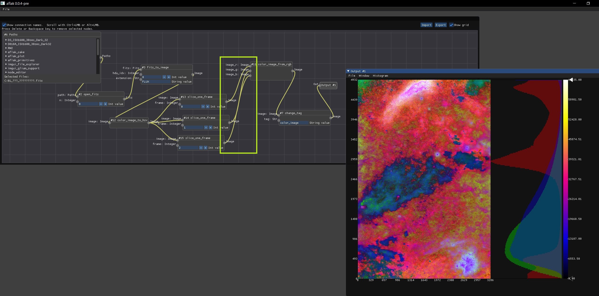
上の図で,HをR,SをG,VをBに接続していることが表現されています.
トーンカーブの作成
お次はトーンカーブ.ゼロから作らなければならなかったので,これが一番面倒でした.まずはインタフェースからのんびり作っていきます.
#[derive(Clone, Debug, Serialize, Deserialize, PartialEq)]
pub struct ToneCurveState {
  arr: Vec<f32>,
  cp: Vec<[f32; 2]>,
  adding: Option<[f32; 2]>,
  pushed: bool,
  moving: Option<usize>,
  deleting: Option<usize>,
  x_clicking: usize,
  is_dragging: bool,
}

impl ToneCurveState {
  pub fn default() -> Self {
    /*省略*/
  }

  pub fn control_points(self) -> Vec<[f32; 2]> {
    self.cp
  }

  pub fn array(self) -> Vec<f32> {
    self.arr
  }
}

impl PartialEq for ToneCurveState {
  fn eq(&self, val: &Self) -> bool {
    let cp1 = self.control_points();
    let cp2 = val.control_points();
    cp1 == cp2
  }
}

pub trait UiToneCurve {
  fn create_curve(cp: &Vec<[f32; 2]>) -> Vec<f32>;
  fn tone_curve(
    &self,
    state: &mut ToneCurveState,
    draw_list: &WindowDrawList,
  ) -> io::Result<Option<ToneCurveState>>;
}

impl<'ui> UiToneCurve for Ui<'ui> {
  fn create_curve(cp: &Vec<[f32; 2]>) -> Vec<f32> {
    /*省略*/
  }

  fn tone_curve(
    &self,
    state: &mut ToneCurveState,
    draw_list: &WindowDrawList,
  ) -> io::Result<Option<ToneCurveState>> {
    let p = self.cursor_screen_pos();
    let mouse_pos = self.io().mouse_pos;
    let [mouse_x, mouse_y] = [mouse_pos[0] - p[0] - 5.0, mouse_pos[1] - p[1] - 5.0];
    state.arr = Self::create_curve(&state.cp);
    self.invisible_button(im_str!("tone_curve"), [410.0, 410.0]);
    self.set_cursor_screen_pos(p);
    PlotLines::new(self, im_str!("Tone Curve Test"), &state.arr)
        .graph_size([410.0, 410.0])
        .scale_min(0.0)
        .scale_max(256.0)
        .build();
    self.set_cursor_screen_pos(p);
    self.invisible_button(im_str!("tone_curve"), [410.0, 410.0]);
    if let Some(adding) = state.adding {
      let x = adding[0] * 400.0 + 5.0 + p[0];
      let y = (1.0 - adding[1]) * 400.0 + 5.0 + p[1];
      draw_list.add_circle([x, y], 5.0, 0xFF00_FFFF).build();
    }
    let mut counter = 0;
    for i in &state.cp {
      let x = i[0] * 400.0 + 5.0 + p[0];
      let y = (1.0 - i[1]) * 400.0 + 5.0 + p[1];
      if (x - mouse_pos[0]) * (x - mouse_pos[0]) + (y - mouse_pos[1]) * (y - mouse_pos[1])
          < 25.0
      {
        draw_list.add_circle([x, y], 5.0, 0xFF00_00FF).build();
        if self.is_mouse_clicked(MouseButton::Left) && state.adding == None {
          state.moving = Some(counter);
        }
        if self.is_mouse_clicked(MouseButton::Right) {
          self.open_popup(im_str!("delete-control-point"));
          state.deleting = Some(counter);
        }
      } else {
        draw_list.add_circle([x, y], 5.0, 0xFFFF_FFFF).build();
      }
      counter += 1;
    }
    self.popup(im_str!("delete-control-point"), || {
      if MenuItem::new(im_str!("Delete Control Point")).build(self) {
        if let Some(key) = state.deleting {
          state.cp.remove(key);
          state.deleting = None;
        }
      }
    });
    if self.is_item_hovered() {
      if self.is_mouse_clicked(MouseButton::Left) && state.moving == None {
        if !state.is_dragging {
          state.is_dragging = true;
        }
      }
      if state.is_dragging {
        if state.pushed == false {
          state.pushed = true;
          state.cp.push([mouse_x / 400.0, (400.0 - mouse_y) / 400.0]);
        }
        state.adding = Some([mouse_x / 400.0, (400.0 - mouse_y) / 400.0]);
        let lastidx = state.cp.len() - 1;
        state.cp[lastidx] = state.adding.unwrap();
        if state.x_clicking > 255 {
          state.x_clicking = 255;
        }
        if !self.is_mouse_down(MouseButton::Left) {
          state.cp.sort_by(|a, b| a[0].partial_cmp(&b[0]).unwrap());
          state.adding = None;
          state.is_dragging = false;
          state.pushed = false;
        }
      }
      if let Some(key) = state.moving {
        state.cp[key] = [mouse_x / 400.0, (400.0 - mouse_y) / 400.0];
        if !self.is_mouse_down(MouseButton::Left) {
          state.moving = None;
        }
      }
    }
    let state = state.clone();
    Ok(Some(state))
  }
}
まだハードコードされているところとかがあり,要修正ですが貼っておきます.曲線の計算には現在 Catmull-Rom Spline 曲線を使っています.state にはコントロールポイントやルックアップテーブルの配列データ(現在大きさは256,0.0~256.0までの値が格納)が入っていて,次のように使います.
let tone_curve_state = ui.tone_curve(&mut state, &draw_list);
if let Ok(state) = tone_curve_state {
  let state = state.unwrap();
  let control_points = state.control_points();
  let array = state.array();
}
次に,トーンカーブのデータ型を作って,画像データとトーンカーブデータから適用後の画像を出力するノードを作って完成です.
トーンカーブデータのところは省略します.
fn run_apply_tone_curve(image: &WcsArray, tone_curve: ToneCurveState) -> Result<IOValue, IOErr> {
  let mut image_arr = image.scalar().clone();
  let table = tone_curve.array();
  let table_size = table.len() - 1;
  image_arr.par_map_inplace(|v| {
    let key = (*v * table_size as f32 / 65535.0) as usize;
    let value = 65535.0 * table[key] / table_size as f32;
    *v = value;
  });
  Ok(IOValue::Image(WcsArray::from_array(Dimensioned::new(
    image_arr,
    Unit::None,
  ))))
}
ちなみに par_map_inplace という関数は ndarray_parallel という crate にあるもので,中の計算を並列処理してくれます.
普通に map で計算する場合と時間を比較するとこんな感じです.
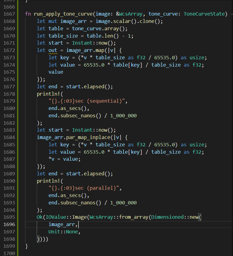 画像にて失礼….
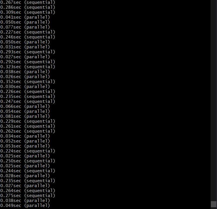 実行結果はこんな漢字です.
結構速くなってますね.他にも直せるところがあると思っています.
さて,数日かけて色々とやりましたが次は何をしましょうか.悩み中です.しばらくは改善とリファクタリングですかね….
なにか作って欲しいものやアドバイスがありましたらブログや Twitter で募集しております.
それでは.